A table cell in TX Text Control ActiveX can calculate its own text: you give it a formula with the TableCellFormula property, and the cell displays the result of the calculation. The property addresses the cell by its table identifier, row and column.

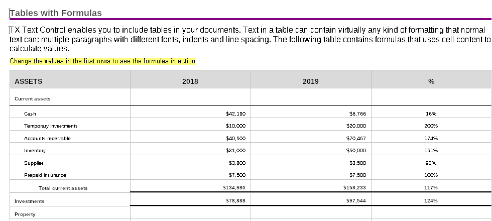
A table of the TXWords demo document whose cells calculate totals and percentages with formulas.

Users enter a formula on the Formulas tab of the Table Properties dialog box that TableAttrDialog opens, and choose the A1 or R1C1 reference style there:

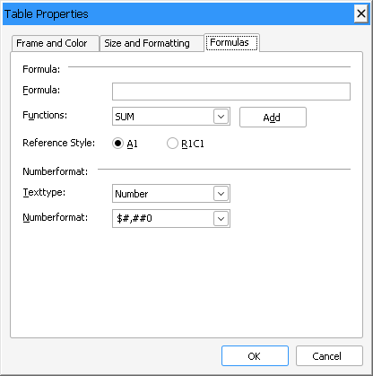
The Formulas tab of the built-in Table Properties dialog box of TXTextControl with the formula, the functions list, the reference style and the number format.

The syntax of these formulas mostly follows the formula specification of SpreadsheetML (Office Open XML File Formats, ISO/IEC 29500-1, chapter 18.17.2 Syntax), which most spreadsheet applications, such as Microsoft Excel, also use. If you have written spreadsheet formulas before, the constants, operators, functions and cell references below will look familiar.

How a Formula Is Built

A formula can consist of four kinds of elements: functions, cell references, constants and operators. The first three represent values inside the formula. Operators connect these elements and perform the calculation or operation.

The following sample formula contains a function, a cell reference, a constant and two operators:

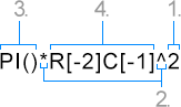
The sample formula with its four parts numbered: 1 the constant 2, 2 the caret and multiplication operators, 3 the function PI and 4 a relative R1C1 cell reference.

Constant. 2 is a number constant.
Operators. ^ is the caret operator. It raises the value of the table cell referenced by R[-2]C[-1] to the power of 2. The * operator multiplies the result of this calculation by Pi.
Function. PI() is a function that returns the value of Pi: 3.14159265.
Cell reference. R[-2]C[-1] returns the value of the table cell two rows above and one column to the left of the formula's table cell.

Use Constants

A constant is a value that doesn't change and can be part of a formula. TX Text Control supports five types of constants: numerical, logical, string, error and array constants.

Numerical Constants

A numerical constant is an integer (for example 4), a decimal number (for example 3.937) or a number in engineering notation (for example 5e4). It can have a minus sign in front of it (for example -7.6).

Formula	Result
`9+7`	16
`4*5.5`	22
`4*3e5`	1200000
`-9+7`	-2

Logical Constants

There are two logical constants: TRUE and FALSE.

Formula	Result
`15>7=TRUE`	TRUE
`15>7=FALSE`	FALSE

String Constants

A string constant is a sequence of characters in double quotes.

Formula	Result
`"TX"&"Text"&"Control"`	TXTextControl
`"Two"="One"`	FALSE
`"FALSE"="FALSE"`	TRUE

Array Constants

An array constant represents a matrix of numerical, logical or string constants, or a mix of them. The constants of a row are separated by commas and the rows by semicolons. Braces enclose the array constant.

Formula	Result
`SUM(10,{1,2,3;4,5})`	25

Combine Values With Operators

An operator applies an operation to the formula elements next to it. TX Text Control supports three groups of operators:

Arithmetic operators perform mathematical operations. Their result is a numerical value.
Comparison operators result in a logical value.
The text concatenation operator joins strings.

Arithmetic Operators

Arithmetic operator	Example
`+` (addition)	The formula `8+6` returns 14.
`-` (subtraction)	The formula `14-6` returns 8.
`*` (multiplication)	The formula `4*3` returns 12.
`/` (division)	The formula `17/2` returns 8.5.
`%` (percent)	The formula `290%` returns 2.9.
`^` (exponentiation)	The formula `3^2` returns 9.

Comparison Operators

Comparison operator	Example
`=` (equal to)	The formula `2=2` returns TRUE.
`>` (greater than)	The formula `4>6` returns FALSE.
`<` (less than)	The formula `4<6` returns TRUE.
`>=` (greater than or equal to)	The formula `6>=4` returns TRUE.
`<=` (less than or equal to)	The formula `26<=4` returns FALSE.
`<>` (not equal to)	The formula `2<>2` returns FALSE.

Text Concatenation Operator

Text concatenation operator	Example
`&` (concatenation)	The formula `"TX"&"Spell"` returns TXSpell.

Call Functions

TX Text Control provides predefined functions that perform specific calculations. The result of a function is always a number, a logical value, a string or an array of such values.

A function begins with its unique name in uppercase letters, followed by an opening parenthesis, the arguments it needs separated by commas, and a closing parenthesis:

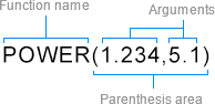
The function POWER(1.234,5.1) with its function name, its two arguments and the parenthesis area labeled.

Valid arguments are numerical, logical, string and array values. You can give them as constants, as the result of another function or as a reference to another table cell.

Function	Example
`ABS(x)`: computes the absolute value of x	`ABS(-7.765)` results in 7.765.
`PI()`: returns the value Pi	`PI()` results in 3.141592654.
`POWER(x,y)`: computes x raised to the power y	`POWER(3,2.5)` results in 15.5884573.
`SUM(argument-list)`: adds the numeric values of the arguments in argument-list	`SUM(1,2,3)` results in 6.
`SUM(argument-list)` with an array constant	`SUM({1;2;3})` results in 6.
`SUM(argument-list)` with a cell reference range	`SUM(A1:A3)` results in 6 if the table cells A1, A2 and A3 hold the values 1, 2 and 3.

The Supported Formula Functions section lists every function, grouped into Mathematical and Trigonometric, Statistical, Logical, Lookup and Reference and Information functions.

Refer to Other Table Cells

A formula often needs the values of other table cells, as an element of the formula or as an argument of a function. TX Text Control provides two styles of cell references, the R1C1 style and the A1 style, and the FormulaReferenceStyle property determines which of them a formula uses.

R1C1 Style

An R1C1 cell reference gives the row as R and a number and the column as C and a number. These numbers can be relative or absolute.

The relative R1C1 style is the one TX Text Control recommends for cell references. A relative reference puts the numbers in square brackets, and they count rows and columns from the table cell in which the formula is defined.

In the following table, a formula is defined in the fourth row (R4) of the third column (C3):

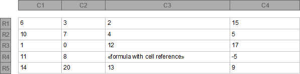
A table of five rows and four columns, labeled R1 to R5 and C1 to C4, with a formula with a cell reference in the cell at R4 and C3 and numbers in the other cells.

Relative R1C1 reference	Description
`R[-3]C[-1]`	Refers to the table cell in the first row (R1) and the second column (C2), with the value 3.
`R[1]C[-2]`	Refers to the table cell in the fifth row (R5) and the first column (C1), with the value 14.
`R[0]C[1]`	Refers to the table cell in the same row (R4) and the fourth column (C4), with the value -5.
`R[-2]C[1]`	Refers to the table cell in the second row (R2) and the fourth column (C4), with the value 5.

An absolute R1C1 reference has no square brackets around its numbers. It always refers to the same cell position, no matter in which table cell the formula is defined: R5C4 is always the cell in the fifth row and the fourth column. Absolute R1C1 references are supported, but don't use them if the table is edited or the part of the table that contains them is pasted as a new table. In these cases, an absolute R1C1 reference returns invalid or incorrect values.

A1 Style

An A1 cell reference gives the column in uppercase letters (A to Z, then AA to AZ, BA to BZ and so on; the first column is A, the second B) followed by the row as an integer. B3 refers to the table cell in the second column and the third row. This notation is a relative cell reference and is the equivalent of the relative R1C1 style.

To make an A1 reference absolute, put a $ sign to the left of the column, the row or both. An absolute reference does not depend on the table cell in which the formula is defined.

Cell Reference Ranges

Some functions accept an argument list with any number of values. If these values are in table cells, adding the references one by one is inconvenient. A cell reference range defines a matrix of table cells instead: two cell references separated by a colon, the first for the upper left and the second for the lower right corner of the range.

The following table applies four ranges to the SUM function in a formula defined in the cell at R3 and C3:

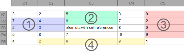
A table of five rows and five columns with a formula with a cell reference at R3 and C3 and four highlighted, numbered ranges of cells: 1 from R2C1 to R3C2, 2 from R1C3 to R2C3, 3 from R1C5 to R4C5 and 4 from R5C2 to R5C4.

Formula with cell reference range	Description
1. `SUM(R[-1]C[-2]:R[0]C[-1])`	Sums the values between R2C1 and R3C2 and returns 16.
2. `SUM(R[-2]C[0]:R[-1]C[0])`	Sums the values between R1C3 and R2C3 and returns 14.
3. `SUM(R[-2]C[2]:R[1]C[2])`	Sums the values between R1C5 and R4C5 and returns 20.
4. `SUM(R[2]C[-1]:R[2]C[1])`	Sums the values between R5C2 and R5C4 and returns 19.

LEFT, ABOVE and RIGHT

The flags LEFT, ABOVE and RIGHT are another way to specify a cell reference range. Each of them refers to the cells next to the formula's table cell in its direction: SUM(ABOVE) sums the values of all cells above the formula's table cell.

The following table applies the three flags to the SUM function in the cell at R3 and C3:

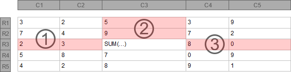
A table of five rows and five columns with SUM(...) in the cell at R3 and C3 and three highlighted, numbered ranges: 1 the cells to the left of it, 2 the cells above it and 3 the cells to the right of it.

Formula with cell reference range	Description
1. `SUM(LEFT)`	Sums the values to the left of the formula's table cell and returns 5.
2. `SUM(ABOVE)`	Sums the values above the formula's table cell and returns 14.
3. `SUM(RIGHT)`	Sums the values to the right of the formula's table cell and returns 8.

Using Formulas in Table Cells